[Excel小技巧:凍結窗格] 讓欄位標題固定位置、不隨著捲動!
「凍結窗格」是微軟Excel軟體中相當好用的功能,在OpenOffice軟體裡也有同樣的功能,凍結窗格功能可以幫我們將Excel文件中指定的欄或列設定在固定位置,當我們上下或左右捲動頁面時,被「凍結」的欄位標題或相關敘述都可以保持在原本的位置,不會因為捲動到其他位置而消失在螢幕範圍中,方便我們快速對照、瀏覽同一份文件前後端的相關訊息。
這應該也是很多人都知道的小技巧,,
先看一下設定「凍結窗格」效果的DEMO影片:
一、Excel 2003的「凍結窗格」使用方法:
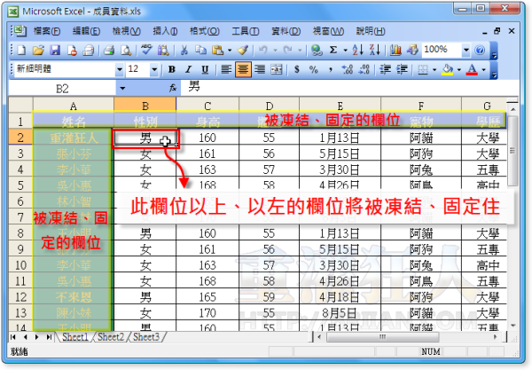
第1步 開啟Excel文件,在你要凍結的欄位的「下一個」窗格點一下。舉例來說,如果你要讓「列1」這一列的資料固定位置、不隨著捲動的話,請點選「列2」這個列裡的任何一個窗格,如「A2」或「B2」...等。
如果你要讓「欄A」這一欄的資料固定位置的話,請點選「B」這一欄中的任何一個窗格,如「B1」或「B2」…等。如果你要同時讓「列1」與「欄A」同時固定位置、不隨著捲動的話,請點選「B2」這個窗格。
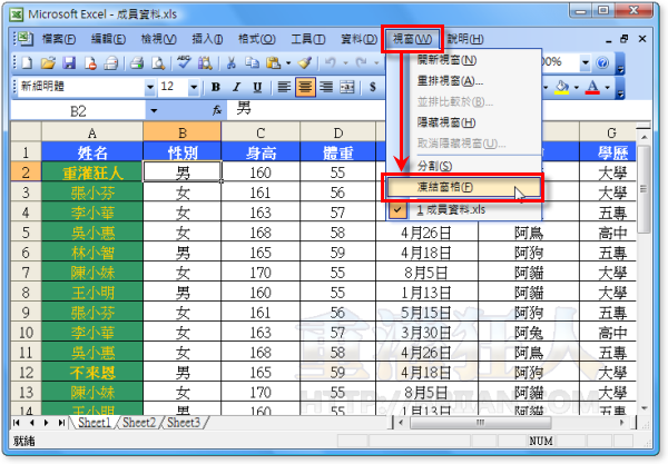
第2步 選取好凍結的窗格後,請依序按下〔視窗〕→【凍結窗格】,接著你的資料表便可像上面影片那樣,不管怎麼捲動頁面中的資料「列1」與「欄A」都會固定不動。
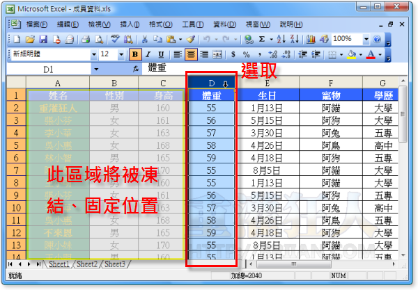
第3步 如果你要讓A、B、C等欄中的資料固定位置、不捲動,請選取整個D欄,然後再按〔視窗〕→【凍結窗格】,這樣只有A、B、C三個欄位中的資料會固定位置不捲動,「列1」的資料則可隨著捲動。設定哪個窗格或欄位要被凍結可以依照自己的需求隨時設定、修改。
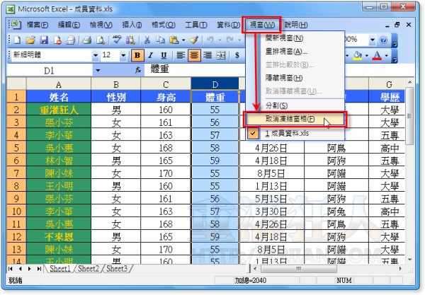
第4步 如果要取消凍結窗格的話,請依序按下〔視窗〕→【取消凍結窗格】即可。
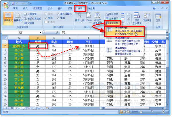
二、Excel 2007的「凍結窗格」使用方法:
在Office 2007版軟體裡面的Excel的操作方法也是一樣,只是功能擺在不同位置而已。
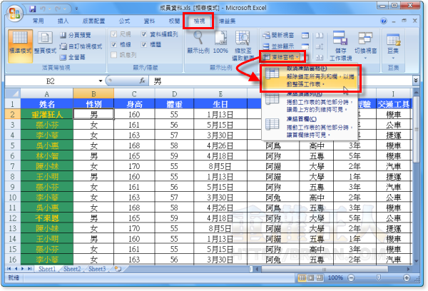
第1步 用Excel 2007開啟文件後,先切換到〔檢視〕這個功能頁面,先點選你要凍結的窗格後,依序按下「凍結窗格」→「凍結窗格」即可。
第2步 如果要取消的話,一樣是按「凍結窗格」→「取消凍結窗格」。
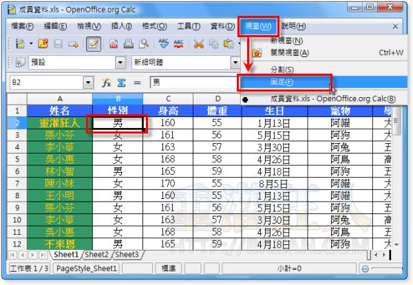
三、OpenOffice Calc的「固定」使用方法:
在OpenOffice的Calc軟體中,「凍結窗格」功能稱為「固定」,同樣是放在「視窗」下拉選單中,一樣是先點選你要凍結的窗格,然後再按下〔視窗〕→【固定】即可。
感謝布萊恩大大,分享這麼實用的功能!雖然很簡單,但是很多人都不知道有這個功能!!
感謝!
如果是活頁簿
每張活頁簿都凍結第一至第四列
而第一至第二表頭部份不顯示出來
譬如列一是**股份有限公司
列二是99年發票明細表
列三是發票一些資料表頭
要如何使列一至列二不出現在每張活頁簿
列三凍結
但列印時還可以列印出列一至列二
請問 在GOOGLE使用時 他只能凍結5欄 有辦法再多幾欄嗎?
Google Document 的解決辦法
Here is a script I use; I started with the custom date format script and added freezing columns/rows. Puts a toolbar button up, “Format & Freeze”; columns and rows are selected separately. For no frozen rows or columns, enter 0.
Not sure if you need help loading the script, but just in case (and for others):
From your spreadsheet -> Tools -> Script Editor -> when the window opens, delete the default Function myFunction() { }; if you already have scripts, you can do Script Manager -> then select New and delete the default function stuff -> Copy the script below -> Paste into the project window you have open -> Hit Save -> Name your script -> Hit OK -> Close the project -> Re-load your sheet. You should now see the Format & Freeze button.
Note: If you are running multiple onOpen scripts, you may need to adjust your triggers.
function onOpen() {
var ss = SpreadsheetApp.getActiveSpreadsheet();
var menuEntries = [ {name: “Change cell format”, functionName: “EditFormat”},
{name: “Reset format to default”, functionName: “ResetFormat”},
{name: “Freeze Columns”, functionName: “FzColz”},
{name: “Freeze Rows”, functionName: “FzRowz”},
]
ss.addMenu(“Format & Freeze”, menuEntries);
}
function EditFormat() {
var oldname = SpreadsheetApp.getActiveRange().getNumberFormat();
var name = Browser.inputBox(“Current format (blank = no change):\r\n”+ oldname);
SpreadsheetApp.getActiveRange().setNumberFormat((name==””)?oldname:name);
}
function ResetFormat() {
SpreadsheetApp.getActiveRange().setNumberFormat(“0.###############”);
}
function FzColz() {
var oldname2 = SpreadsheetApp.getActiveSheet().getFrozenColumns();
var name2 = Browser.inputBox(“Current frozen columns (blank = no change):\r\n”+ oldname2);
SpreadsheetApp.getActiveSheet().setFrozenColumns((name2==””)?oldname2:name2);
}
function FzRowz() {
var oldname3 = SpreadsheetApp.getActiveSheet().getFrozenRows();
var name3 = Browser.inputBox(“Current frozen rows (blank = no change):\r\n”+oldname3);
SpreadsheetApp.getActiveSheet().setFrozenRows((name3==””)?oldname3:name3);
}
Hope that helps. If you find this helpful, please help out other users by marking the question as answered. Thanks. Dan
謝謝~這個小技巧幫了後大的忙呢!不用再拉上拉下^^~
我只要凍結姓名、姓別、身高那欄是不是就不能??
因為他會自動設行、列到10
gj
大大不好意思…..再加問一個,有辦法整列或整欄儲存格一起設定公式嗎?醬就不用一格一格設定!ㄏㄏㄏ謝謝
這真的超好用的,正好最近整理大量資料,視窗都要一直拉來拉去的,時在省去我不少麻煩!真的太感謝了!!
另外有一問堤想請教大大,我有一欄資料是要輸入年齡,我希望他能隨系統時間而增加,該如何編寫程式呢??謝謝!!
看了回應,果然還是很多人不會。
簡單講
選擇欄,凍結窗格,則被選擇的欄往左方的欄都會凍結
選擇列,凍結窗格,則被選擇的列往上方的列都一起凍結。
選擇儲存格,則儲存格往上方的列及往左方欄都凍結
簡單講會被凍結的區域就是在你現行格的往左往上的區域
感謝老頭子的回覆, 簡單又明暸.
大推 感謝大大
我也不知道這點
今天才知道
XD
真的很實用!
使用這麼多年來第一次學到 = =”
真的不知道,有看過別人用,但沒特別想到要學,所以也沒特別找
…
所以多看是好事,我每天都來增加 pegaview … @@
真的是正好派上用場…..
我一值在找這個功能說=.=+
太感謝啦
很實用的小技巧喔~
(潛水一年多, 第一次發言啦~~呵呵呵~~~)